Ch 07. 로지스틱 희귀(Logistic Regression)
Part.6 Logistic Regression 실습
Logistic Regression
Load Dataset from sklearn
In [1] :
import pandas as pd
import seaborn as sns
import matplotlib.pyplot as plt
In [2] :
from sklearn.datasets import load_breast_cancer
cancer = load.breast_cancer()

print(cancer.DESCR)
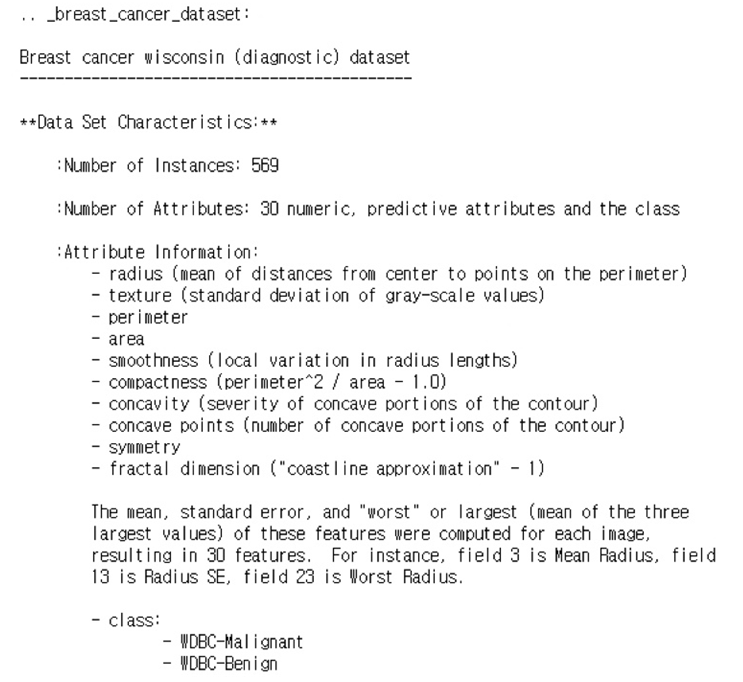
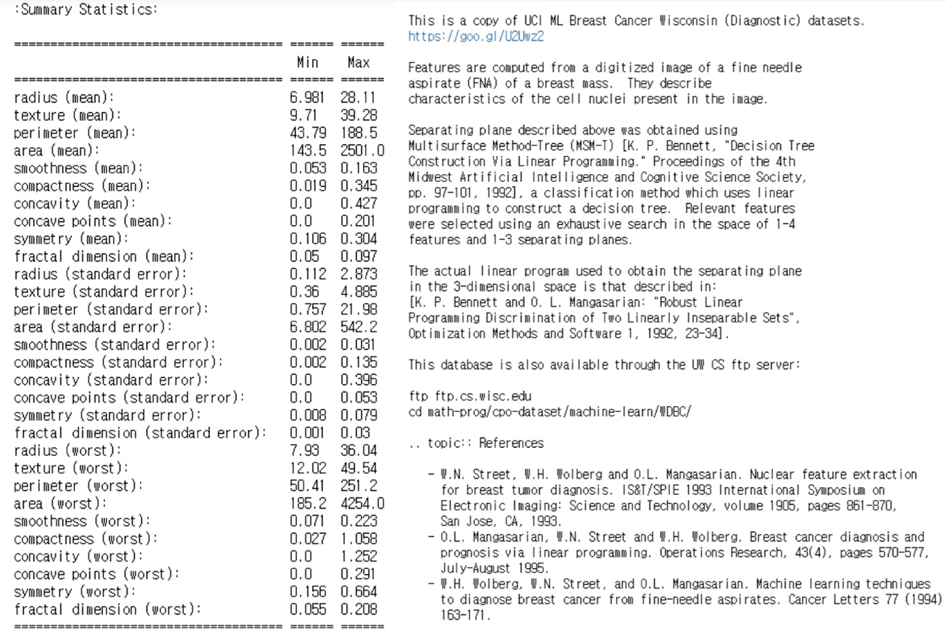
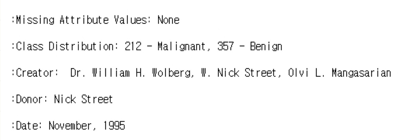
In [3] :
df = pd.DataFrame(cancer.data, colums=cancer.feature_names)
df['class'] = cancer.target

df.tail()
Out [3] :

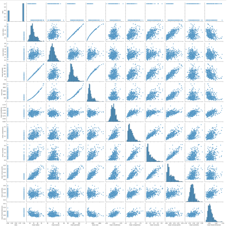
Pair Plot with mean features
In [4] :
sns.pairplot(df[['class'] + list(df.columns[:10])])
plt.show()
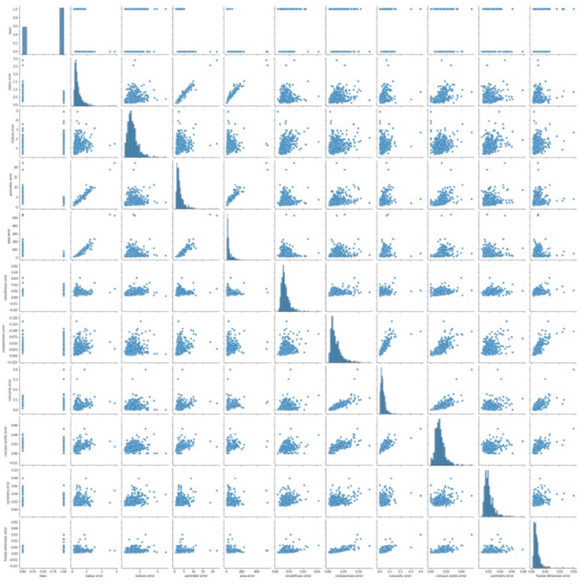
Pair Plot with std features
In [5] :
# 아래로 내려 갈수록 값은 0에 가까워지고, 위로 올라갈수록 1에 가까워진다.
sns.pairplot(df[['class'] + list(df.columns[10:20])])
plt.show()
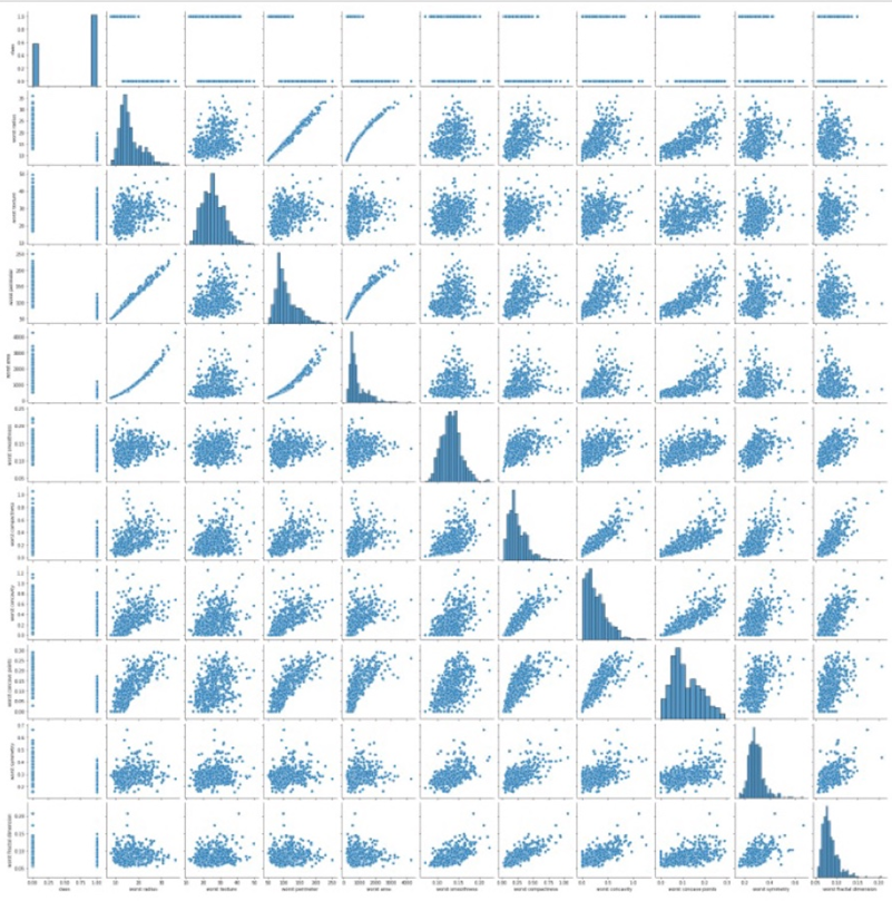
Pair plot with worst features
In [6] :
sns.pairplot(df[['class'] + list(df.columns[20:30])])
plt.show()
Select features
In [7] :
cols = ["mean radius", "mean texture",
        "mean smoothness", "mean compactness", "mean concave points",
        "worst radius", "worst texture",
        "worst smoothness", "worst compactness", "worst concave points",
        "class"]
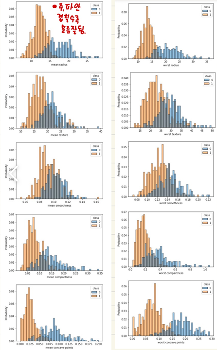
In [8] :
for c in cols[:-1]:
    sns.histplot(df, x=c, hue=cols[-1], bins=50, stat='probability')
    plt.show()
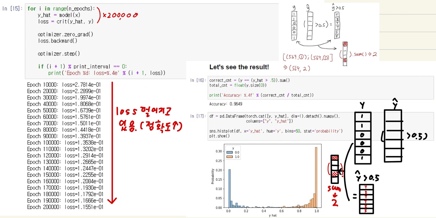
Train Model with PyTorch
####
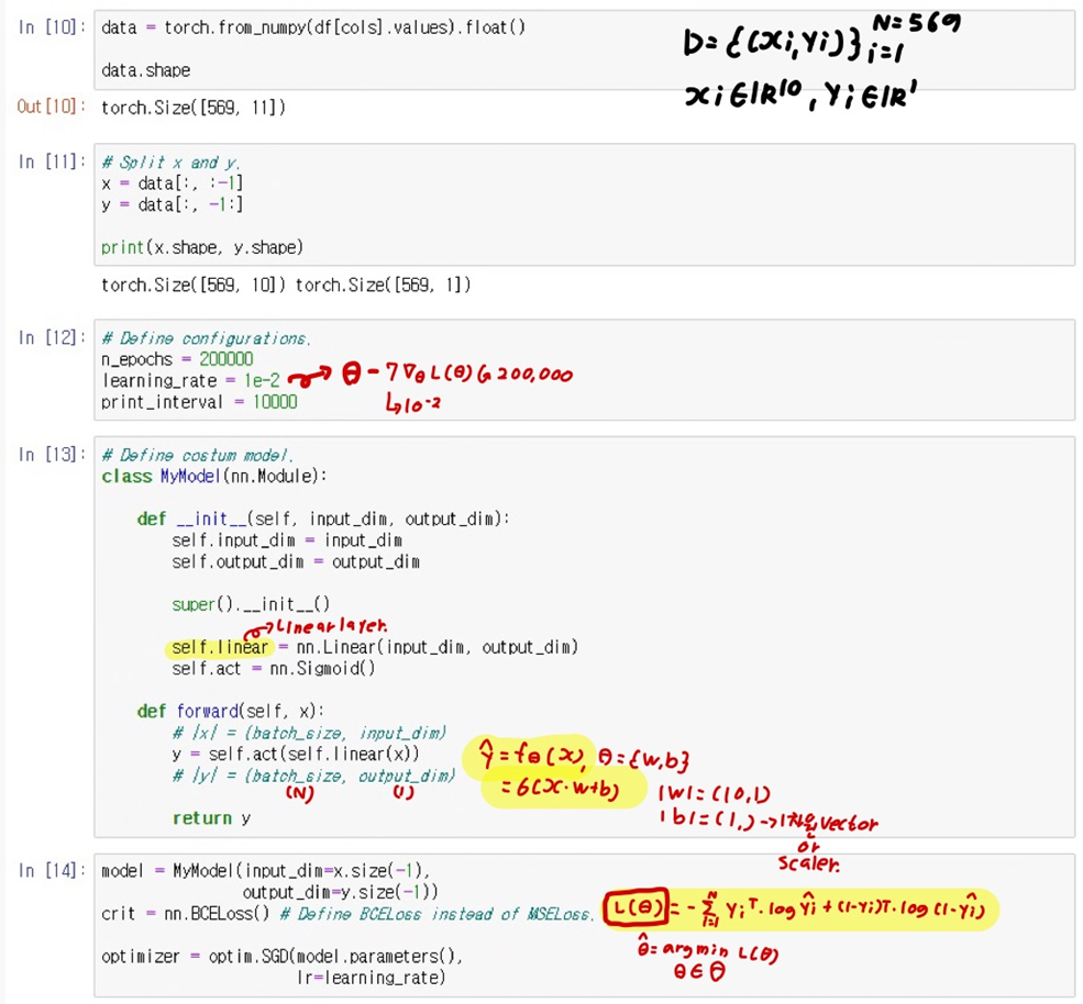
In [9] :
import torch
import torch.nn as nn
import torch.nn.functional as F
import torch.optim as optim
